Continuous Probability Distributions
What is the difference between continuous variables and discrete variables?
A major difference between continuous and discrete random variables is the former takes on uncountable and infinite number of possible outcomes in a given interval. Hence the range of continuous random variable X comprises all real numbers in an interval. In addition to the above given illustrations, water consumption amount in a household, weights of people in a population, the speed of wind in a open certain area, waiting time in a supermarket, checkout lanes or load on a bridge are the few examples for continuous random variable for real world applications. From these examples it’s clear that random variable X can take unaccountably infinite values.
What are the properties of the probability denstiry function of a continuous random variable?
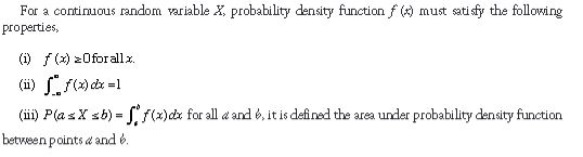
Assume that f(x)=x2/9 is a probability density function for 0≤x≤c. Find the value of c.
Since f(x)=x2/9 is a probability density function it must satisfy:

Thus c=3
Assume that f(x)=x2/9 is a probability density function for the closed interval (0,3). Find P(X>2)

Define the cumulative distribution function.
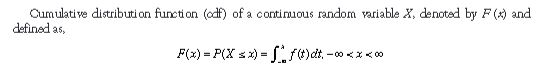
What are the properties of the cumulative distribution function?
Similar to discrete random variables, CDF F (x) of a continuous random variable X, fulfills the following properties:
(i). 0 ≤ F (x) ≤ 1and
(ii). If
x1 ≤ x2 then F (x1) ≤ F (x2)
Find the cumulative distribution function of the PDF f(x)=0.05 for 0 ≤x ≤20.
We will find the cumulative distribution function for 3 intervals.
1. interval:x<0
2. interval: 0 ≤x ≤20
3. interval:x>20
Thus:

Assume that the cumulative distribution function for the random variable x is defined as F(x)=x3 for the interval 0<x<1. Derive the probability density function f(x).
The PDF is the first derivative of the CDF. So:
f(x)=dF(x)/d(x)=3x2
Define the mean, variance and standard deviation of the random continuous variables formally.

Find the mean of the random variable x if the density function is given as f(x)=x2/9 for 0<x<3.

Find the variance of the random variable x if the density function is given as f(x)=x2/9 for 0<x<3.

So variance=27/80
Define uniform distribution.
The probability density function f (x) of the uniform continuous random variable X takes a constant value over the range of the random variable X is defined.
Formally define the uniform distribution function.

Define the mean and variance of the uniform distribution.

Random variable X takes values between 20 and 40. Find the distribution function.
We can use a geometric solution, since the area of the distribution function must be equal to 1. The shape of the uniform distribution is a rectangle as shown below:

thus f(x)=0.05 for 20<x<40
Find the mean and the variance of variable x if it is uniformly distributed between 20 and 40.
the minimum value of x is a=20
the maximum value of x is b=40
Mean=0.5(a+b)=30
Variance=(b-a)(b-a)/12=100/12=25/3=8.3333...
Find P(x<38) if x is uniformly distributed between 20 and 40.
The simpliest solution is geometric. P(x<38) is equal to the area of the rectangle whose short size is 0.05 (1/(40-20)=0.05) and long size is 18 (38-20=18). Thus P(x<38)=0.05*18=0.9
Explain the normal distribution.
Normal distribution is one of the most significant and extensively used continuous probability distribution. The major reason for this circumstance is majority of the continuous random variables which are observed through real life applications (social, medical, physical, biological) are normally or approximately normally distributed (bell-shaped) variables. Furthermore, normal distribution provides basis for the statistical inference. Because of its shape, normal distribution occasionally called “bell curve” or also called “Gaussian curve” which was developed by a mathematician Karl Friedrich Gauss. In addition to common properties of distribution functions:
Normal distribution is symetric around the mean.
The probability density function f (x) does not the touch and intersect x axis.
What is the standard normal distribution?
Standard normal distribution is a special case for the normal distribution where the mean μ=0, the standard deviation σ=1 and denoted as z ~ N (0,1). Probability density function f (z) for the standard normal random variable z can be obtained as follows where the mean μ=0, the standard deviation σ=1 are placed in the normal density function of f (x).
Define the exponential distribution and give examples of it.
Exponential distribution is another most significant and extensively used continuous probability distribution. Exponential random variable is frequently used to model the time interval between two events. Some illustrations of random variables that generally conform to model by means of exponential distribution are presented below.
• Arrival time between two customers.
• Time between two messages.
• Time between telephone calls received by a customer service.
• Time between customers who are arriving to the checkout lane of the supermarket.
• Time between two failures of a certain mechanical device.
Formally define the density function of exponential distribution, its mean and variance.
